Search And Replace

Search And Replace:

If you want to replace all the words before or after a particular word, string, symbol etc.
1- Press CTRL+H, there is a Find and Replace dialogue box will show.

2- Now we have a data of bus terminal names and we want to replace all the data written before terminal.

3- Now in find what field of Search and Replace dialogue box type Terminal and put asterisk<*> symbol before Terminal <*Terminal> and in Replace with field give the value you want, here we give <DTC Terminal>.

5- Click Replace All.

Done.

->And if you want to replace all the data after a particular word, put the asterisk<*> symbol after that particular word.

Now press Replace All and data after Terminal will replace with Terminal

Read More

Vlookup Function

VLOOKUP Function:

The VLOOKUP function searches for a value in the first column of a table array and returns a value in the same row from another column in the table array.
The V in VLOOKUP means "Vertical".

Syntax:- =VLOOKUP(value, table_array, index_number, [not_exact_match])

VLOOKUP is used when your comparison values are located in a column to the left of the data that you want to find.



1. The first column must be in alphabetical or numeric order.
2. The VLOOKUP formula has 4 components:
a. Lookup_value: The value to search in the first column of the table array.
b. Table_array: Two or more columns of data. The values in the first column of table_array are the values searched by lookup_value.
c. Col_index_num:  The column number in table_array from which the matching value must be returned. A col_index_num of 1 returns the value in the first column in table_array; a col_index_num of 2 returns the value in the second column in table_array, and so on.
d.Range_lookup: A logical value that specifies whether you want VLOOKUP to find an exact match or an approximate match. If TRUE or omitted, an approximate match is returned. In other words, if an exact match is not found, the next largest value that is less than lookup_value is returned.  If FALSE, VLOOKUP will find an exact match. If one is not found, the error value #N/A is returned.

VLOOKUP Example Image

3. Enter the formula: =VLOOKUP(A2,H2:I6,2,0)

a. A2 is the look up value.
b. H2:H16 is the range in which you want to find A2 value.
c. 2 is the column number from which matching value which should be returned.
d. 0 stands for exact match.
4. Copy the formula for the rest of the items.

VLOOKUP Example Image

VLOOKUP Image

Note:

1- If the range from which the value is being retrieved is not in order then VLOOKUP will not pick some values.






2- To fix it  so you will have to freez the range.

VLOOKUP

3- Now the result will remain same.

MS Excel VLOOKUP

Read More

Navigating the options with keyboard

For every option there is an access key. Anyone can quickly use a command by pressing a few keys. Every command can be accessed by using an access key. You can get the most commands by using two to five keystrokes. To use an access key:

1. Press ALT key:
The KeyTips are displayed over each option that is available.

2. Press the letter shown in the KeyTip over the feature that you want to use.
3. After pressing the letter which you want, you may be shown additional KeyTips.
4. Continue pressing letters until you press the letter of the command or control that you want to use.

Read More

Macros / How to Record Macros in Excel

MACROS:

Macros is one of the best function in Excel. With the help of Macros you can automate your work. Macro is a set of instructions that tells excel what to do. Macros commands are written in Visual Basic for Applications(VBA) programming language.

Macro function records your actions or commands. Recorded macros can be run whenever you want, automatically repeating your recorded actions and saving your time and effort.

Record a Macro:

Record Macro

Here we try recording a macro to produce your name and address:
1- Go to Developer Tab, click on Record Macro.

* Developer Tab- If Developer Tab is disable you can enable it. To enable Developer Tab click on Office button which is on the most left upper corner then click on Excel Options. On the Popular menu check Show Developer tab in the Ribbon.

2- Enter Macro name as Excel_Add in the Macro name box.
* Macro name should start with alphabets, doesn't accept spaces, instead of space can use ( _ )underscore as a word separator.

3- Enter a shortcut key in Shortcut key box.
* To assign a shortcut key for your macro either you can type a single character(character which is not used already for any shortcut key for excel) or can type with SHIFT key.


4- Leave the setting at This Workbook in the Store macro in box.

5- In Description box, give the description for your macro whatever you want and click OK.

Excel Sheet

6- Now on Sheet1, go to the cell A1 and type your name and address.(You can format your text as you want).
7- Now on the Developer tab click on Stop Recording button.
Now a Macro has been recorded.

Macros

Running a Macro:

To run a macro follow the steps given below:

1- Select the cell where you want to run the record macro. 

2- Go to Developer Tab, click on Macro button. A dialogue box with Macro name will open.

3- Select your macro which you name as Excel_Add and click on Run.

OR
1- You can just simple press your shortcut key which you created at the time of macro recording.

Read More

Introduction to MS Excel

MS Excel Intro

IMPORTANCE OF EXCEL

Excel is the most important computer software program used in workplace today.  This one is the main reason to learn excel in order to enter or remain in the workplace. In the field of information systems excel is used as an end-user computing tool.

Outside the workplace, Excel is also use for everyday problem solving.
Calculation in excel is very easy and effective. With the help of excel, you can calculate the cost of trip by car, can track your income and assets etc.

Excel has become popular and a staple of business professionals as well as end users. Excel is used widely by businesses, volunteer groups, scientists, private sectors organizations, service agencies, educators, accountants, journalists, trainers and many others.

Excel is one of the most important tools of the workplaces so an employer should learn excel.

Read More

Function Wizard & Cell Reference

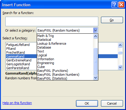
THE FUNCTION WIZARD
There are two ways to insert a function in excel spreadsheet:
1-By typing directly into the cell or in fourmula bar.
2-By using the INSERT FUNCTION option.
There are many ways to accessing the INSERT FUNCTION dialog box: 1-Go to formulas menu and click on INSERT FUNCTION option. 2-Just click on INSERT FUNCTION(fx) icon on formula bar. 3-Press SHIFT+F3
CELL REFERENCES
This is one of the most important thing everyone should know about this.  Three type of cell references are:
1-Relative
In relative reference, column and row numbers change as it copied to other cell respectively.
2-Absolute
In absolute reference, column and row numbers doesn't change wherever it copied in the spreadsheet.
3-Mixed
Mixed reference is the combination of Relative and Absolute
Reference	Cell		Range
Relative	A4		A4:B5
Absolute	$A$4		$A$4:$B$5
Mixed	$A4 or A$4		$A4:B$5
$(Dollar) symbol denotes that the particular cell or range is freezed so no matter where it is copied the values will remain same.
Two ways to freeze cell or range:
1-By directly typing the $ (Dollar) symbol.
2-By press F4
First time when anyone press F4 it freeze both the column and row, second time only row and third time only column. Please leave you comments and suggestion in comment box.

Read More

Numeric/Mathematical Function

Numeric/Mathematic Function-
To know the average value of numbers provided. Average called also arithmetic mean	AVERAGE	=AVERAGE(Number1, Number2, ...Number_n)
To count the number of cell that contains numbers.	COUNT	=COUNT(argument1, argument2, ....argument_n) *argument1, argument2..argument_n can be the ranges or cells or values.
To count the number of cells in a given criteria.	COUNTIF	=COUNTIF(range, criteria)
To count the number of cells in single or multiple criteria.	COUNTIFS	=COUNTIFS(critaria1_range, criteria1, critaria2_range, critaria2,...critaria_n_range, critaria_n)
To find the reminder after a number is devided by a divisor.	MOD	=MOD(numbner, divisor)
To add all numbers in a range of cells.	SUM	=SUM(cell1:cell2, cell3:cell4,...) OR =SUM(number1, number2,...number_n)
To add all numbers in a range of cells based on given criteria.	SUMIF	=SUMIF(range, criteria, [sum_range]) *sum_range is optional(if it is blank function uses range as the sum_range)

Read More

Formulas: String Functions

STRING FUNCTIONS:

To remove all non printable characters.	CLEAN	=CLEAN(text)
To combine two or more strings.	CONCATENATE	=CONCATENATE(text1, text2)
		to combine any specific word use "" (inverted commas) like "excel".
To extract a substring from a string starting from the left-most character.	LEFT	=LEFT(text, no of characters)
To find the length of any specified string.	LEN	=LEN(text)
To convert all the letters in lowercase.	LOWER	=LOWER(text)
To convert all the letters in uppercase.	UPPER	=UPPER(text)
To set the first character in each word to Uppercase	PROPER	=PROPER(text)
To remove all leading and trailing spaces.	TRIM	=Trim(text)
To extract a substring from a string between two specific numbers.	MID	=MID(text, start_position, number_of_characters)
To replace a set of characters with another from a string.	SUBSTITUTE	=SUBSTITUTE(text, old_text, new_text, [starting position])

Read More

Excel Charts And Graphs

Charts

Charts and Graphs
 
 Microsoft Excel lets you turn your raw data into a variety of charts and graphs. Using this feature, you can visually
summarize numerical information and display any trends or
patterns that are present. Charts and graphs can help make your data more meaningful and easier to understand.
When you create a chart or graph, you will have a number of types and styles to choose from. Make sure to choose the chart type that best displays your data. These
are the most commonly used types of charts:

Column Chart

Column:- Column charts are made up of vertical bars representing multiple sets of data. They are most often used to show how amounts have changed over time.

Bar Chart

Bar:- Bar charts are made up of horizontal bars representing
multiple sets of data. They are most often used to compare various amounts at a fixed point in time.

Line Chart

Line:- Line charts are made up of lines representing multiple sets of data. They are most often used to show changes over time and are good for emphasizing trends.

Pie Chart

Pie:- Pie charts are made up of slices representing a single set of data. They are most often used to show how parts relate to the whole.

Read More