Enter Key Movement / How to set Enter key Direction.

How to set Enter key direction in MS Excel? Change cursor position after pressing Enter key on Keyboard in Microsoft Excel. Change Enter key direction Up, Down, Left, Right in Excel spreadsheet or workbook manually.

Every time when we press Enter key on the computer keyboard in Microsoft Excel, the cursor move downwards in the cells. So, Can we change the Enter key behavior / behaviour in Excell?  Suppose every time when you press Enter in MS Excel, you want to move your cursor left, right or up instead of down which is by default in Excel. Is this possible in Excel? The answer is absolutely yes.

Office button

So, changing or setting Enter key direction / behaviour in MS Excel is not a very hard / tough exercise. you can easily change this by follow some of the given steps:-

1) Open your Ms Excel and click on the File Menu in MS Excel 2010, in MS Excel 2007 click on the office button which is in upper left corner of the Excel Spreadsheet or Workbook.

2) Click on the Options menu, a window named as Excel Options will open.

3) Click on the Advanced menu / option.

4) In Editing options, there will be an option- "After pressing Enter, move selection

Direction:"

5) Change or set the direction as per your requirement or you want from the drop down list. Enjoy.

Read More

VLOOKUP / EXCELL VLOOKUP FUNCTION / EXCEL VLOOKUP FORMULA / MS EXCEL VLOOKUP

VLOOKUP / EXCELL VLOOKUP / VLOOKUP FUNCTION / EXCEL VLOOKUP FORMULA / HOW TO USE VLOOKUP IN EXCEL SPREADSHEET? / VLOOKUP EXAMPLE 2007/ VLOOKUP FUNCTION EXAMPLE / VLOOKUP FORMULA EXAMPLE / EXAMPLES OF VLOOKUP / VLOOKUP DESCRIPTION WITH EXAMPLE.

Here we are going to discuss the most important and most useful function / formula of MS Excel i.e VLOOKUP. About every person who works on MS Excel, use VLOOKUP as VLOOKUP is a very useful and powerful function / formula for MS Excel. Basically we use VLOOKUP for put a data or value from another table into one table with the basis of a common value, cell, range or data either the table is from the same spreadsheet or different spreadsheet, or we can say that we fetch a data / value from another table into one table with the help of VLOOKUP FUNCTION in MS Excell. So Here we use VLOOKUP with an example. We discuss, how to use VLOOKUP / Put VLOOKUP in cell or range of cells in Excel Spreadsheet.

Now lets start using VLOOKUP Function / VLOOKUP Formula in Excel, suppose we have two table one is Sales Table which contains sales data of the products and another is Product Table which contains the product information of Products. The Product Name column contains the matched values of products in both the tables.

Table 1:-Sales Table which contains the sales information of the products. There are two columns in Table 1-Sales, Column A is Product Name and Column B is Sales.

Table 2:-
Product Table which contains the Product information of the products. There are two columns in Table 2-Products too. Column A is Product Name and Column B is Product Price.

Now in Table 1-Sales, if we want to insert / fill / fetch product price from Table 2-Product we will have to use MS Excel / Excell VLOOKUP Function / VLOOKUP Formula to fetch or fill the values of product price column in Table 1-Sales from another table 2-Product.

MS Excel VLOOKUP Formula / VLOOKUP Function:-

=VLOOKUP(lookup_value, table_array, col_index_num, [range_lookup]

>Lookup_value is the value to be found in the first column of the table, and it can be value, a reference, or a text string.

Remember:- Lookup_value should be in the left of the data always, vlookup doesn't insert / fill / fetch values in the left hand side from the lookup_value.

>Table_array is a table of text, numbers, or logical values, in which data is retrieved, Table_array can be a reference to a range or a range name

>Col_index_num is the column number in table_array from which the matching value should be returned. The first column of values in the table is column 1.

>Range_lookup is a logical value: to find the closest match (approx match) in the first column (sorted in ascending order)=TRUE or omitted; find an exact match = FALSE.

Note:- we can write 1 instead of TRUE in range_lookup and can write 0 instead of FALSE in range_lookup. It's a time consuming activity in Excel VLOOKUP Formula.

Now in Table 1-Sales give Column C name Product price and write the VLOOKUP formula as:-

=VLOOKUP(A3,Products!A3:B9,2,0)

In this Formula:-

A3 is the lookup value which is being search in table 2-Products.

Products!A3:B9 is the range of table from which we want to insert / fetch / fill the data.

2 is the column_index_num, which column value we want. First we select a range of table from A3 to B9 in this total no of Row are from 3-9 means 6 rows and Column from A-B means 2 Columns and we want 2nd column (B Column value) so here we put 2 as a column_index_num.

0 is the range_lookup, we want here exact match so we write 0.

Read More

Flag Duplicate Values Automatically / Find Duplicate Values Automatically

Automatically Flag Duplicate Values On Input / Know Duplicate Values Automatically while Inputing Value / Find Duplicate Values Automatically in Excel

Sometimes you may be a requirement of preventing duplicates values from being entered in a range of cells in excel worksheet. Enabling this capability in Excel is not tough.

Here is how we can automatically flag duplicate values while inputing values in a specific range of cells in your excel worksheet. Follow the given below method to implement this:-

1) Select the range of cells where you want to prevent duplicate values (e.g. C3:C20);

2) Click on Data Validation button in the Data Tools group From the Data tab;

3) Click the Allow drop-down and select Custom from the list on the Settings tab. A Formula field will appear;

4) Type =COUNTIF($C$3:$C$20,C3)<2 in the Formula field. When you will enter the data into a cell, this formula will be  evaluated. If the formula will evaluate / return to TRUE, the entered value will be accepted. The formula in this example says, count how many times the Active Cell's value appears in the range C3:C20. If it will less than 2, will allow it, otherwise, the Error Alert message will display which you entered. In this example, C3 is the Active Cell. You will need to adjust your formula as required. It is critical that you use Absolute referencing for your validation range (e.g. $C$3:$C$20) and relative referencing for your Active Cell (e.g. C3);

5) Click the Input Message tab, in the Data Validation dialog and, if desired, type a message that will be displayed when the user selects a cell within the range of the Data Validation rule. Otherwise, if you don't want a message to appear every time someone selects a cell in the range, clear the 'Show input message...' option.

6) Click the Error Alert tab and type the message that will be displayed if the user enters a duplicate value in the range;

7) Click OK.

Now test your Data Validation rule by entering values, including some duplicates, within the range.

Edit or Delete Existing Data Validation Rules:-
 
To edit or delete existing validation rules, you start by selecting a cell within the validation range. Note that the formula in the Data Validation dialog will now be relative to the currently active cell. To ensure that the rule is applied to all of the cells in the validation range, select the 'Apply these changes to all other cells with the same settings' option before clicking OK.

How to find / know for which cells you have been applied Data Validation Rules:-
After you have applied Data Validation rules to your worksheet, you may not remember for which cells or range you have applied Data Validation rules to. Thankfully, there is an simple method to find the Data Validation rules in your Excel worksheet.

Finding ranges containing Data Validation:
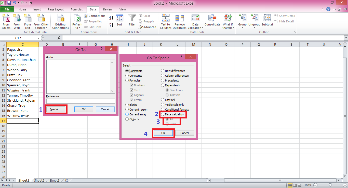
1) Press the F5 key on your keyboard;

2) click the Special... button which is on the GoTo dialog;

3) In the bottom right corner of the dialog select the Data Validation option. Click All to select all Data Validation ranges in the worksheet or Same to highlight just the cells that have the same Data Validation rules as the active cell.

NOTE:-
But, there is one major drawback when using Data Validation. It does not stop a user from pasting invalid data into the range. When pasting into a cell containing Data Validation, the validation is removed because the cell's formatting is overwritten. For the most part, however, Data Validation is very useful for preventing invalid entries.

And as you can see in the Settings tab of the Data Validation dialog, there are many other validation options that you can apply to your data.

Read More

How to AutoFill values when adjacen column contains Blanks

How to AutoFill values when adjacent / side column contains Blanks. Simple Solution to AutoFill Issue When Adjacent Column Contains Blanks. Fill values automatically when adjacent / side column contains blanks.

How to AutoFill data in a column?

One of Excel's coolest features is Double-clicking the fill handle. It is the fastest way to fill formulas down a long column. It can AutoFill hundreds or even thousands of numbers or dates or formulas in a split second. I don’t think that Excel users are not aware of this.

Now suppose you 1000 records in a excel worksheet and there is a value in the adjacent cell and you want to fill it till the end of the Data (1000 Records). You just double click the right lower corner of the cell and the data will be automatically filled. But if you have blank cells in the middle of the data then data will not fill till the end of the data. When you double-click the Fill Handle, AutoFill stops dead in it's tracks if there are blank cells in the adjacent column.

So, how to fill the data automatically even if the adjacent column have blank cells in the data?

Here is a very simple and easy trick to update / fill the values automatically even if the adjacent column has blank cells in the data.

One alternative, is to select the first cell containing the formula to be filled down, drag the vertical scrollbar to move quickly down to the last row, hold down the SHIFT key and click the last cell you want to fill. This will select all cells from the first to the last cell. Then press CTRL+D to copy the formula to all the selected cells.

Here is an easier way by hiding Column(s).

If there are blank cells in an adjacent column preventing the double-click AutoFill from working, a quick workaround is to hide the column(s) containing blank cells until you have an adjacent column that is completely filled and then use the double-click fill method as usual.

NOTE:- Don't forget to unhide your column(s).

Read More

How to select & delete blank cells in between data in Excel

Select and Delete blank cells in between data in Excel. How to select blank cells to delete in between the data within a worksheet in Excel?
 
Sometimes we have a large data with some blank values and we need to delete all these blank rows or columns from the worksheet in Excel and it's not so simple to delete the blank rows and column by selecting one by one. If we have records in lacs then it might take a whole day or more or you can get frustrate too. So here is a very simple trick to select the blank cells (rows or columns) within the data and delete all those at once.

I) Put your cursor within the data range and press CTRL+G, the Go To dialog box will open then click on Special button (Alternatively you can click the 'Go To...' or 'Go to Special...' option in drop down list of Find & Select option in Editing group of Home tab).
 

II) Now Select Blanks and Hit Enter. All the blank cells within the data will be selected. 
 
III) Now press CTRL+-(minus) or Right click above any selected cells and click on Delete.
 

IV) A Delete dialog box will open with four option:

->Shift cells left
->Shift cells up
->Entire row
->Entire column

Select either shift cells up or Entire row and Hit ok.

Rememer:- There may be a discrepancy in order of your data if a single cell is blank with data in next cell, either complete row will be deleted or can change the order of your data.

Read More

Delete ALT+ENTER / Line Breaks in Excel

How to insert next line in a cell in excel, Insert line break in excel, Remove ALT+ENTER Special character, Delete ALT+ENTERed symbol, Remove line break, Easiest way to delete ALT+ENTER / line breaks or Special Character (CHAR(10).

Sometimes you need to insert a next line in a cell in Excel, but when you press Enter, it moves into  the next cell so what should we do to insert a line break / new line in a cell in MS Excel. To insert a new line / line break you will have to press ALT+ENTER whenever you want to enter a new line or line break in a cell in MS Excel.
Now here is a very important question, if we want to remove or delete this line break / new line and want to have text in a single line, what we can do?
When we press ALT+ENTER a new special character is inserted at that place, to remove that special character we can use methods.

So, if you want to get rid of the line break or remove the special character which occured when you press ALT+ENTER you can simply click immediately before the line break and press Delete button or click immediately after the line break and press Backspace button.

But if you have a worksheet that has a lot of cells that contains line breaks or lets say this special character and you need to delete (get rid of line breaks)  that special character or line break from the cells in MS Excel, you will not use Delete button or Backspace button because it's not a right exercise or a time consuming exercise. Is macro required for this exercise, No!

Here are some methods to delete / remove line break / ALT+ENTER special character:-

1:- Using Find & Replace:
By using Find & Replace method you can quickly get rid of all those line breaks in your worksheet. If you want to remove or delete line breaks or ALT+ENTERed special character from only part of the worksheet, select that range first, otherwise select any single cell. Then

I) Press CTRL+H (Keyboard shortcut for FIND & SELECT And REPLACE), You can open FIND & REPLACE dialog box by going to Home tab and select REPLACE from the drop down option of FIND & SELECT which is in EDITING group.

 
II) Click in the 'Find What' field, hold down the ALT key and type 0010 (only using the numeric keypad) and release the ALT key. It may looks like nothing in the 'Find What' field but you have actually entered an invisible (line break) character.

NOTE:- You can use CTRL+J instead of ALT+0010 in 'Find What' field. This shortcut is easier to remember or use.

III) Click in the 'Replace with' field, press the spacebar once or any character or word you want to replace ALT+ENTER with and click the Replace All button.

2:- Remove, replace or delete manual new line / line breaks in Excel cells by using Wrap Text.

Remember that Excel automatically applies Wrap Text to cells when a forced line break is inserted, so to remove the wrapped text formatting go to the the Home tab and click Wrap Text in Alignment group.

It may not be apparent but you may have caused some cells to have two blank spaces. You can easily find and Delete, Remove, Replace or get rid of them by using Find & Replace, just enter the two blank spaces in the 'Find What' field and replace it with one blank space in 'Replace with' field.

3:- Remove, Delete ALT+ENTER (get rid of line breaks) Using a Formula:
You can also use a formula to remove / delete line breaks (ALT+ENTER character).
Here is a very interesting formula given below:  
 
I) =SUBSTITUTE(A1,CHAR(10)," ")
Use this formula to replace manual line breaks in Excel cells.
How it does work?(How to use substitute function in Excel or how substite work in Excel)?

Actually Substitute function replace an old character or word with a new word or charcter you want.
=SUBSTITUTE(text, old text, new_text, [nth_appearence or instance number])
Here:

A1 =  text (in which you want to replace, remove or delete ALT+ENTER / line break)
 
CHAR(10) = special character code for ALT+ENTER
 
 " " =  New text "Space" (Replace ALT+ENTER / line break with space)
 
nth_Appearence  or instance number = used when you want to replace or remove the Nth number of Character or Word(Lets say if you have two ALT+ENTER or two line breaks in a cell and you want to remove, replace or delete only first or second ALT+ENTER /  line break then just give Nth_appearence (Instance Number) 1 if you want to replace first ALT+ENTER /  line break or give Nth_appearence (Instance Number) 2 if you want to replace second ALT+ENTER /  line break).

NOTE:- You can also use =SUBSTITUTE(A1,"  "," ") to replace double blank spaces with single blank spaces, use two spaces inside double quotes instead of CHR(10) in the previous formula in place of FIND & REPLACE method.

II) Use Clean function to remove / Delete ALT+ENTER / line breaks in EXCEL:

Using CLEAN function is also one of the easiest way to remove, replace or delete ALT+ENTER character / symbol or line break in Excel Cells.
=CLEAN(A1)
Remember by using CLEAN function you can't add another character, string, symbol or word in place of ALT+ENTER /  line breaks.

Read More

Trick to Sort / Order Dates By Month And Day (Ignoring Year).

How to sort dates data by month and day / Sort dates by month and day / Ignoring year sort dates by months & dates, Trick to Order by or Sort Dates by Month And Day.

Sometimes you need to sort dates by month and day while ignoring the year, such as grouping anniversary dates (e.g Employees, Clients, Birthdays etc....).
When you will sort dates in a column they will be sorted by year, by default. If there will dates from multiple years and you want your data arranged by months, there will no obvious solutions for this type of sorting.

Here is a solutions for sorting dates by months and day. As there are so many methods to do one work in excel, here are also other ways to do this, but this one is quick and simple.
Lets do it.

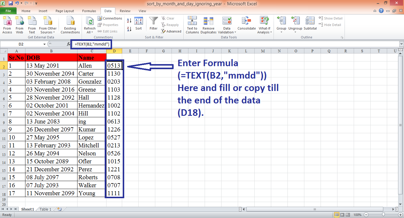
1) Now I have some data (Range-A1:C18) in which I have Names and their Date of Birth (just for an example). Now This data is sorted by names or order by names, what I have to do, sort the date with months and dates except years (ignoring year in date).

2) In a blank column (D2), enter the following formula.

=TEXT(A4,"MMDD")

3) Fill this formula down to the bottom of your data (D18);

4) Now select the complete date from starting to the end (A1:D18) and apply sorting (go to Data tab, click on Sort button in Sort & Filter group, there a dialog box named Sort will opened, Select (Column D) in sort by field and click ok.

Now the data has been sorted or ordered by Month & Date without / except years (or Ignoring year).

Hope this will help you, don't forget to leave your suggestions and feedback in comment box.

Read More

Hiding A Cell's Contents / Simple Tricks For Hiding a Data of a Cell / Hide Data in Excel/ Protect Sheet/ Worksheet in Excel

Hiding A Cell's Contents / Simple Tricks For Hiding a Data of a Cell / Hide Data in Excel/ How to hide data cells from printing in Excel?, Protect Sheet / Spreadsheet in Excel.

In Excel sometimes we want to hide data or content of cells. Suppose you have some data / value in your excel spreadshet but you do not want to be displayed or printed, then what you will do for this, perhaps you will store these values / data in some far corner of the worksheet, in a hidden row or column, or even storing them on another worksheet. Here is a question is there only these ways to do so or there is any other simple option or trick, the answer is yes there is a very simple trick to do so.

How to hide a content, data, value of a cell or multiple cells in excel spreadsheet?
How to hide cells from printing in Excel?Here are a some tricks that you may want to try instead.
>> One simple and a very easy is to simply change to font color for those cell to match the background color of your worksheet (Usually it remains white), thereby making the cell contents invisible.

>> The second trick is very good and interesting you certainly like it. So to simply hide the value by applying a special custom number formating code to the cells. Follow the given below steps:

1) Select the cells you wish to hide;

2) Now open Format Cells dialog box (To open Format Cells dialog box you can simply press CTRL+1);

3) Now Go to the Number tab and select Custom from the given Categories;

4) In the Type box (Right ahead the Categories), enter ;;; (three semicolons);

Now what the ;;; (three semicolons ) number formatting code tells to the Excel?
It tells to the Excel that if the cell contents /  data or value are either a positive number, a negative number, a zero value or a text, display nothing.

Note :- But Here a catch, when a cell is selected the contents are visible in the Formula bar, so to hide it permanently or to hide a cells contents in the Formula Bar, you need to protect your sheet. To protect your sheet follow these given steps:

To hide a cells contents in the Formula Bar...

Before going to protect your sheet in excel, you need to change the Hidden property of the cells. 

1) Select the cells you want to hide from the Formula Bar;

2) On the Home tab click Format in the Cells group;

3) Click the Protection tab and place a checkmark in the Hidden property;

4) Go to the Review tab, click Protect Sheet in the changes group, in Protect Sheet dialog box give a password you want to give and check only uppermost two option and leave rest of all unchecked.

Hope this will help you. Please leave your suggestions, feedback in comment box.

Read More

CTRL+.(Dot) Excel Shortcut Key / Know the last or first cell of the selected or filled data in Excel.

How to know the last cell of selected or filled data / CTRL+.(Dot) Key Shortcut Excel / Know the range of filled data or selected data in Excel with Example.

MS Excel is a very big and useful software which use in almost every company or firm. Those people who do work on excel, they select data or fill data many times in a day or in their work period either it is vertical or horizontal or a set of rows and columns, everyone use shortcuts to select data or fill data (by double click the lower right corner on the cell) like CTRL+Down Arrow Key or CTRL+END key. So if we want to know how much data or records have been selected, how can we find.
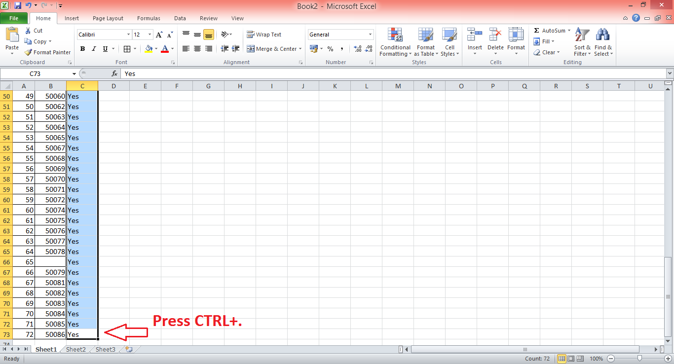
Here is an amazing trick or you can say a shortcut, when you have selected or filled your data just press CTRL key with . (Dot) key i.e (CTRL+.) and you will reach the bottom cell of the selected data or records, once again if you press CTRL+. then you will reach the top cell of the selected data. Isn't it very interesting and useful, check it yourself and use it.

EXAMPLE:

Now we have a data and we want to fill a status column with Yes value just for example, there are almost 73 records in this worksheet.

We don't know how far the value will be filled automatically so after filling the status column, to fill automatically value double click the lower right corner of the cell.

And to find out how far the value has been filled we just press CTRL+.(Dot) and here we see the cursor is in the last cell till where the data has been filled.

Try yourself and enjoying. Don't forget to leave your suggestions or comments.

Read More

Trace Formula In Excel/ Audit Formulas in Excel

Auditing Formula in Excel/ Trace Formula in Excel/ Know dependency of cell on other cells in Excel/ Display the relationships between formulas and cells.

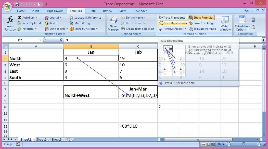
When you are working with a worksheet that has a lot of formulas and  there is a concern sometimes is that what will happen to a lot of formulas if we change a cell or cell value. For example in Cell B2 has the value 9 and C8 has the formula that contains the cell B2 or it's value.

If we change that B2 value which is 9 then the formula in C6 will react, now we also concern about other cells might react if we change B2, for doing this manually we have to worry about which cells will change if B2 changes in that sheet or other sheets in the workbook which relates to the value of B2 or C8.

Tracking down this manually is almost unthinkable, so it's good to find out those cells which depends on B2 and it's not so tough or hard to locate or find out the dependancy of cell B2.

On the Formulas tab in the ribbon we got the choice in the Formulas Auditing group there is an option of Trace Dependents, it will help to find out the dependency of a cell value on the other.
So first put your cursor on cell B2 and then click on Trace Dependents then you will see an arrow pointing towards that cell which depends on Cell B2, so by this you can find out those cells which will react if you change any cell or it's value.

By this tool you can find the dependency of a Formula or a cell in Excel. For more information regarding this you can go to the Microsoft Office official website: http://office.microsoft.com/ or click here to go directly to Microsoft website.

Read More

Format Multiple Cells at Once/ Format Painter Multiple Cells Excel

Copy format into multiple cells with Format Painter/ How to Format Multiple Cells at Once/ Apply format of a cell into multiple cells with Format Painter.

Format Painter is a very useful tool, if you want to copy a format of a cell and want to apply it on another cell, go to the formated cell and click on Format Painter tool which you will find on Home tab just below the copy button. Now click wherever you want to apply or paste that format.

Format Painter Button

But how to format multiple cell at once in excel, is it possible with Format Painter? The answer is yes, it is possible.
It's very simple, go to the formated cell and after that double click on Format Painter. Now you can apply that format into multiple cells. It's a very simple and time consuming activity. Try it.

Format Painter

Read More

Pivot Table Excel

Pivot Table:


Pivot Table is one of the most powerful tools of excel. Infact, justice to pivot tables cannot be done by using more words however, it is one of "the more you sink yourself, the more you challenge yourself" kind of a tool.
It is a tool which helps a user in analyzing and summarizing data and presenting it in a customized way. The USP (Unique Selling Point) of Pivot tables is that one can select a considerable data from huge data sets in performing various activities like (business) analytics, business intelligence, reporting etc.

To give an overview, once data has been selected, one needs to choose the option of Insert (in the ribbon) and then Pivot table (given at top left). Once we set up the Pivot table, we can simply drag and drop fields in various options given at the right which otherwise would have been by use of different formulae.
Therefore, Pivot table not only gives a deep consideration to aesthetics but also saves a millenia by avoiding to type the formulae in analyzing data sets.

Read More

Hlookup Function/ Hlookup Formula with Example

Hlookup Formula with example:

An advice - if one asserts to be an excel user and is sincere in his claims, then you just can't get without saying - "i don't know the lookup family in excel".
Vlookup and hlookup are the lynchpins of matching data. The alphabets "v" and "h" stand for vertical (lookup) and horizontal (lookup) respectively.
Talking about hlookup in this section, its use is less when compared to vlookup since data sets have columns arranged vertically, however, if one has read my first line, one just cannot abandon it.

The syntax for hlookup is - (lookup_value,table_array,row_index_num,[range_lookup]). To avoid you from scrtaching heads, please look below to decipher what the syntax means -
lookupvalue - value that needs to be searched in the first row
table_array - cell ran
ge  or name of the table that contains both the value to look up and the related value to return
row_index_num - serial number of the row whose value you want to return
[range_lookup] - An optional logical argument which is either TRUE or False;
TRUE - for an exact match
FALSE - for an appropriate match

HLOOKUP Example:

We have a data of sales of four regions months wise and we want the sale value in B2 cell of East Region in February 2014. Write [=HLOOKUP(B1,$B$5:$E$7,3,FALSE)] formula in B2 Cell and we can find the East Region sale value of February Month 2014 from the Sales data.

Read More

Offset Function/ Offset Formula Excel

Offset:

If the hlookup and vlookup belong to one family then one can say Match and Offset belong to the other one.

Offset is a pretty simple formula to be used in excel. However, as a suggestion from my end, one needs to use it in small data workbooks else, it becomes pretty tricky.

The syntax and its description is given below -

Offset(reference, rows, cols, [height], [width]) where,

reference - is a (output) cell or a range of adjacent cells from which you want to base the offset

rows - stands for no. of rows one wants to move up or down from the reference cell. +ve value denotes moving down and vice-versa

columns - stands for no. of coolumns one wants to move right or left from the reference cell. +ve value denotes moving right and vice-versa

[height] - which is optional and represents the number of rows selected. it has to be a positive value.

[width] - which is optional and represents the number of columns selected. it has to be a positive value.

Read More

Index Function/ Index Formul Excel

Index:


One propensitates towards complacency after learning the lookups, match, Sumif, Countif etc. because all these are day to day functions and one feels good about himself especially after he/she is tending towards being a rising star in the eyes of his reporting boss.
However, to get the respect which the "Halley's comet" gets, one needs to think out-of-the-box kinds so that he/she can also become like the force of attraction despite the sky being filled with beautiful stars.
To achieve that "Halley's commet" status - learn Index in Excel. It is one of those which can startle you and many others.
It works like any other data retrieving function but it has lot to offer beyond its main function as it can be combined with other functions in excel. There are two sytanxes for an index function which are explained below -


1)INDEX(array, row_number, [column_number]) where,
array - specific range of cells (or can be an entire table)
row_number - the value of the row number that one is wanting to retrieve
[column_number] - which is optional and is the value of the column number that one is wanting to retrieve.

2)INDEX(reference, row_number, [column_number], [area_number]) where,
reference - which means a range that needs to be specified
row_number - the value of the row number within the range that one is wanting to retrieve
[column_number] - which is optional and is the value of the column number within the range that one is wanting to retrieve.
[area_number] - which is optional and is the range that needs to be used from the reference parameter

Read More

If Function/ If Formula Excel

If:
"Ifs" and "Buts" only call the satan and by using If, you can think of all satanically conditional work that can be done in excel.
It is simple and easy to use and the output is all the more pleasing. So let me hurry up with the syntax -
if(logical_test, [value_if_true], [value_if_false]) where,
logical_test - which is nothing but the condition

[value_if_true] - is optional and returns the decided value when the condition is met
[value_if_false]  - is optional and returns the decided value when the condition is not met  

Read More

Match Function/ Match Formula Excel

Match:

Supposedly one is in a real hurry ( i think this needs not to be "supposed" as we have already been made to swallow that time = money), one needs to find the relative position of specific item in a speific range in excel.
In such cases, Match comes into play which is pretty self - explanatory and easy to understand.
The syntax and its description is given below -

Match(lookup_value, lookup_array, [match_type]) where,
lookup_value - is the specific item one is looking for
lookup_array - the specific range of excel
[match_type] - which is optional and gives the value as per type selected which can be either exact match or an appoximate match.

Read More

How to find duplicate words or value in a cell in excel with example.

How to find duplicate words in a cell in excel with example?

To find a duplicate value or word in a cell in excel we can use IF function with SUBSTITUTE function. Now suppose a data contains addresses and we want to know either that data contains duplicate word in a cell or not, so we will use IF with SUBSTITUTE.
We have a file which contain some data of State, City and Addresses.

We wants to find is there any duplicate city name exist in address column or not.

Now in cell D2 we will type formula as =IF(SUBSTITUTE(C2,B2,"",2)=C2,"","Dups") and fill the formula till the end of the data.

In D column there is remark "Dups" for the addresses which contain city name twice.

Explaination:- In Formula (=IF(SUBSTITUTE(C2,B2,"",2)=C2,"","Dups")), First the SUBSTITUTE function replace the city name (city name on the second position, will not replace city name which is on first place because in SUBSTITUTE function we provide the Instance No as 2) which is in city column (B Column) and if substitute the result will match with C column data it means no changes will occur means no city name is on second place in address data but if the substitute result will not match with C column data it means the city name on second position is exist. So if substitute result will not match with C column data there is a remark dups will be filled in D column else it will remain blank.

Read More