How to select & delete blank cells in between data in Excel

Select and Delete blank cells in between data in Excel. How to select blank cells to delete in between the data within a worksheet in Excel?
 
Sometimes we have a large data with some blank values and we need to delete all these blank rows or columns from the worksheet in Excel and it's not so simple to delete the blank rows and column by selecting one by one. If we have records in lacs then it might take a whole day or more or you can get frustrate too. So here is a very simple trick to select the blank cells (rows or columns) within the data and delete all those at once.

I) Put your cursor within the data range and press CTRL+G, the Go To dialog box will open then click on Special button (Alternatively you can click the 'Go To...' or 'Go to Special...' option in drop down list of Find & Select option in Editing group of Home tab).
 

II) Now Select Blanks and Hit Enter. All the blank cells within the data will be selected. 
 
III) Now press CTRL+-(minus) or Right click above any selected cells and click on Delete.
 

IV) A Delete dialog box will open with four option:

->Shift cells left
->Shift cells up
->Entire row
->Entire column

Select either shift cells up or Entire row and Hit ok.

Rememer:- There may be a discrepancy in order of your data if a single cell is blank with data in next cell, either complete row will be deleted or can change the order of your data.

Read More

Delete ALT+ENTER / Line Breaks in Excel

How to insert next line in a cell in excel, Insert line break in excel, Remove ALT+ENTER Special character, Delete ALT+ENTERed symbol, Remove line break, Easiest way to delete ALT+ENTER / line breaks or Special Character (CHAR(10).

Sometimes you need to insert a next line in a cell in Excel, but when you press Enter, it moves into  the next cell so what should we do to insert a line break / new line in a cell in MS Excel. To insert a new line / line break you will have to press ALT+ENTER whenever you want to enter a new line or line break in a cell in MS Excel.
Now here is a very important question, if we want to remove or delete this line break / new line and want to have text in a single line, what we can do?
When we press ALT+ENTER a new special character is inserted at that place, to remove that special character we can use methods.

So, if you want to get rid of the line break or remove the special character which occured when you press ALT+ENTER you can simply click immediately before the line break and press Delete button or click immediately after the line break and press Backspace button.

But if you have a worksheet that has a lot of cells that contains line breaks or lets say this special character and you need to delete (get rid of line breaks)  that special character or line break from the cells in MS Excel, you will not use Delete button or Backspace button because it's not a right exercise or a time consuming exercise. Is macro required for this exercise, No!

Here are some methods to delete / remove line break / ALT+ENTER special character:-

1:- Using Find & Replace:
By using Find & Replace method you can quickly get rid of all those line breaks in your worksheet. If you want to remove or delete line breaks or ALT+ENTERed special character from only part of the worksheet, select that range first, otherwise select any single cell. Then

I) Press CTRL+H (Keyboard shortcut for FIND & SELECT And REPLACE), You can open FIND & REPLACE dialog box by going to Home tab and select REPLACE from the drop down option of FIND & SELECT which is in EDITING group.

 
II) Click in the 'Find What' field, hold down the ALT key and type 0010 (only using the numeric keypad) and release the ALT key. It may looks like nothing in the 'Find What' field but you have actually entered an invisible (line break) character.

NOTE:- You can use CTRL+J instead of ALT+0010 in 'Find What' field. This shortcut is easier to remember or use.

III) Click in the 'Replace with' field, press the spacebar once or any character or word you want to replace ALT+ENTER with and click the Replace All button.

2:- Remove, replace or delete manual new line / line breaks in Excel cells by using Wrap Text.

Remember that Excel automatically applies Wrap Text to cells when a forced line break is inserted, so to remove the wrapped text formatting go to the the Home tab and click Wrap Text in Alignment group.

It may not be apparent but you may have caused some cells to have two blank spaces. You can easily find and Delete, Remove, Replace or get rid of them by using Find & Replace, just enter the two blank spaces in the 'Find What' field and replace it with one blank space in 'Replace with' field.

3:- Remove, Delete ALT+ENTER (get rid of line breaks) Using a Formula:
You can also use a formula to remove / delete line breaks (ALT+ENTER character).
Here is a very interesting formula given below:  
 
I) =SUBSTITUTE(A1,CHAR(10)," ")
Use this formula to replace manual line breaks in Excel cells.
How it does work?(How to use substitute function in Excel or how substite work in Excel)?

Actually Substitute function replace an old character or word with a new word or charcter you want.
=SUBSTITUTE(text, old text, new_text, [nth_appearence or instance number])
Here:

A1 =  text (in which you want to replace, remove or delete ALT+ENTER / line break)
 
CHAR(10) = special character code for ALT+ENTER
 
 " " =  New text "Space" (Replace ALT+ENTER / line break with space)
 
nth_Appearence  or instance number = used when you want to replace or remove the Nth number of Character or Word(Lets say if you have two ALT+ENTER or two line breaks in a cell and you want to remove, replace or delete only first or second ALT+ENTER /  line break then just give Nth_appearence (Instance Number) 1 if you want to replace first ALT+ENTER /  line break or give Nth_appearence (Instance Number) 2 if you want to replace second ALT+ENTER /  line break).

NOTE:- You can also use =SUBSTITUTE(A1,"  "," ") to replace double blank spaces with single blank spaces, use two spaces inside double quotes instead of CHR(10) in the previous formula in place of FIND & REPLACE method.

II) Use Clean function to remove / Delete ALT+ENTER / line breaks in EXCEL:

Using CLEAN function is also one of the easiest way to remove, replace or delete ALT+ENTER character / symbol or line break in Excel Cells.
=CLEAN(A1)
Remember by using CLEAN function you can't add another character, string, symbol or word in place of ALT+ENTER /  line breaks.

Read More

Trick to Sort / Order Dates By Month And Day (Ignoring Year).

How to sort dates data by month and day / Sort dates by month and day / Ignoring year sort dates by months & dates, Trick to Order by or Sort Dates by Month And Day.

Sometimes you need to sort dates by month and day while ignoring the year, such as grouping anniversary dates (e.g Employees, Clients, Birthdays etc....).
When you will sort dates in a column they will be sorted by year, by default. If there will dates from multiple years and you want your data arranged by months, there will no obvious solutions for this type of sorting.

Here is a solutions for sorting dates by months and day. As there are so many methods to do one work in excel, here are also other ways to do this, but this one is quick and simple.
Lets do it.

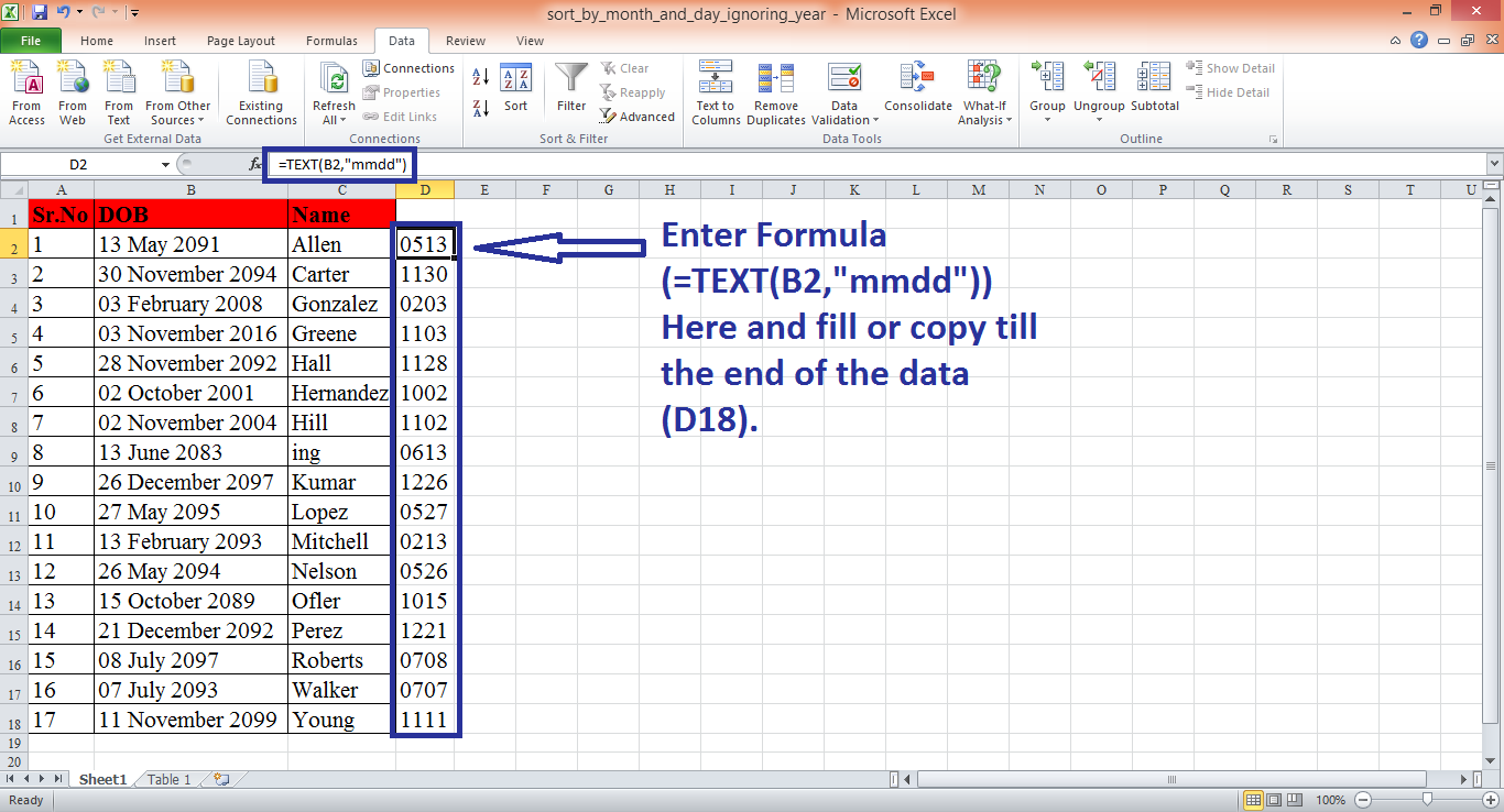
1) Now I have some data (Range-A1:C18) in which I have Names and their Date of Birth (just for an example). Now This data is sorted by names or order by names, what I have to do, sort the date with months and dates except years (ignoring year in date).

2) In a blank column (D2), enter the following formula.

=TEXT(A4,"MMDD")

3) Fill this formula down to the bottom of your data (D18);

4) Now select the complete date from starting to the end (A1:D18) and apply sorting (go to Data tab, click on Sort button in Sort & Filter group, there a dialog box named Sort will opened, Select (Column D) in sort by field and click ok.

Now the data has been sorted or ordered by Month & Date without / except years (or Ignoring year).

Hope this will help you, don't forget to leave your suggestions and feedback in comment box.

Read More

Hiding A Cell's Contents / Simple Tricks For Hiding a Data of a Cell / Hide Data in Excel/ Protect Sheet/ Worksheet in Excel

Hiding A Cell's Contents / Simple Tricks For Hiding a Data of a Cell / Hide Data in Excel/ How to hide data cells from printing in Excel?, Protect Sheet / Spreadsheet in Excel.

In Excel sometimes we want to hide data or content of cells. Suppose you have some data / value in your excel spreadshet but you do not want to be displayed or printed, then what you will do for this, perhaps you will store these values / data in some far corner of the worksheet, in a hidden row or column, or even storing them on another worksheet. Here is a question is there only these ways to do so or there is any other simple option or trick, the answer is yes there is a very simple trick to do so.

How to hide a content, data, value of a cell or multiple cells in excel spreadsheet?
How to hide cells from printing in Excel?Here are a some tricks that you may want to try instead.
>> One simple and a very easy is to simply change to font color for those cell to match the background color of your worksheet (Usually it remains white), thereby making the cell contents invisible.

>> The second trick is very good and interesting you certainly like it. So to simply hide the value by applying a special custom number formating code to the cells. Follow the given below steps:

1) Select the cells you wish to hide;

2) Now open Format Cells dialog box (To open Format Cells dialog box you can simply press CTRL+1);

3) Now Go to the Number tab and select Custom from the given Categories;

4) In the Type box (Right ahead the Categories), enter ;;; (three semicolons);

Now what the ;;; (three semicolons ) number formatting code tells to the Excel?
It tells to the Excel that if the cell contents /  data or value are either a positive number, a negative number, a zero value or a text, display nothing.

Note :- But Here a catch, when a cell is selected the contents are visible in the Formula bar, so to hide it permanently or to hide a cells contents in the Formula Bar, you need to protect your sheet. To protect your sheet follow these given steps:

To hide a cells contents in the Formula Bar...

Before going to protect your sheet in excel, you need to change the Hidden property of the cells. 

1) Select the cells you want to hide from the Formula Bar;

2) On the Home tab click Format in the Cells group;

3) Click the Protection tab and place a checkmark in the Hidden property;

4) Go to the Review tab, click Protect Sheet in the changes group, in Protect Sheet dialog box give a password you want to give and check only uppermost two option and leave rest of all unchecked.

Hope this will help you. Please leave your suggestions, feedback in comment box.

Read More

CTRL+.(Dot) Excel Shortcut Key / Know the last or first cell of the selected or filled data in Excel.

How to know the last cell of selected or filled data / CTRL+.(Dot) Key Shortcut Excel / Know the range of filled data or selected data in Excel with Example.

MS Excel is a very big and useful software which use in almost every company or firm. Those people who do work on excel, they select data or fill data many times in a day or in their work period either it is vertical or horizontal or a set of rows and columns, everyone use shortcuts to select data or fill data (by double click the lower right corner on the cell) like CTRL+Down Arrow Key or CTRL+END key. So if we want to know how much data or records have been selected, how can we find.
Here is an amazing trick or you can say a shortcut, when you have selected or filled your data just press CTRL key with . (Dot) key i.e (CTRL+.) and you will reach the bottom cell of the selected data or records, once again if you press CTRL+. then you will reach the top cell of the selected data. Isn't it very interesting and useful, check it yourself and use it.

EXAMPLE:

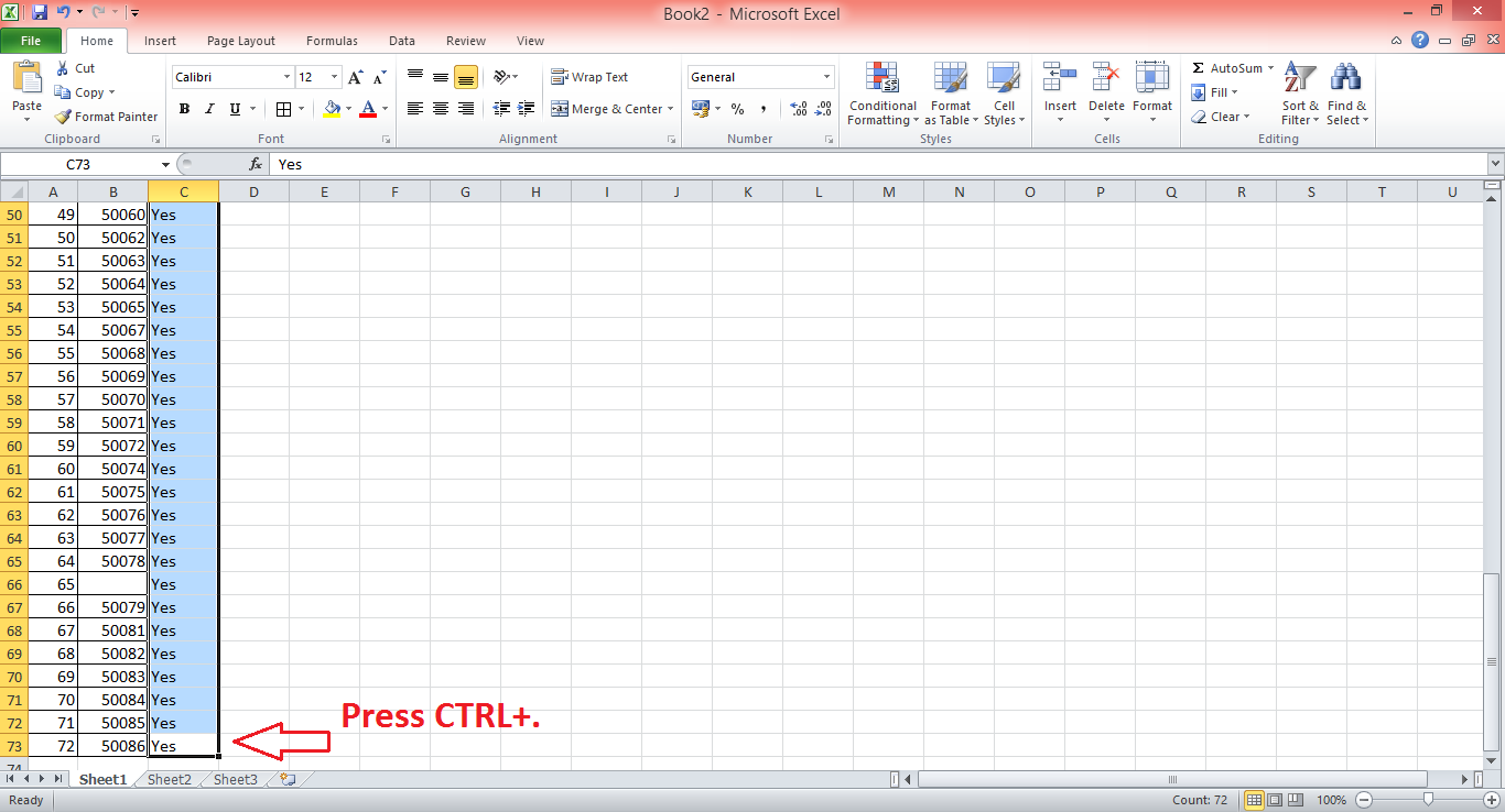
Now we have a data and we want to fill a status column with Yes value just for example, there are almost 73 records in this worksheet.

We don't know how far the value will be filled automatically so after filling the status column, to fill automatically value double click the lower right corner of the cell.

And to find out how far the value has been filled we just press CTRL+.(Dot) and here we see the cursor is in the last cell till where the data has been filled.

Try yourself and enjoying. Don't forget to leave your suggestions or comments.

Read More

Trace Formula In Excel/ Audit Formulas in Excel

Auditing Formula in Excel/ Trace Formula in Excel/ Know dependency of cell on other cells in Excel/ Display the relationships between formulas and cells.

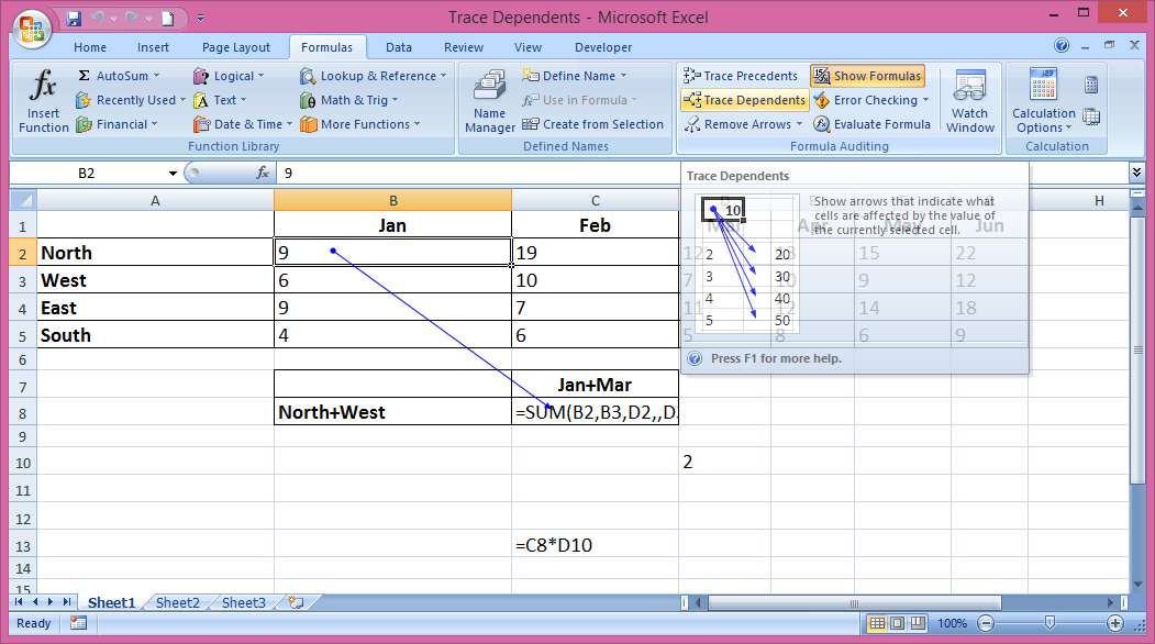
When you are working with a worksheet that has a lot of formulas and  there is a concern sometimes is that what will happen to a lot of formulas if we change a cell or cell value. For example in Cell B2 has the value 9 and C8 has the formula that contains the cell B2 or it's value.

If we change that B2 value which is 9 then the formula in C6 will react, now we also concern about other cells might react if we change B2, for doing this manually we have to worry about which cells will change if B2 changes in that sheet or other sheets in the workbook which relates to the value of B2 or C8.

Tracking down this manually is almost unthinkable, so it's good to find out those cells which depends on B2 and it's not so tough or hard to locate or find out the dependancy of cell B2.

On the Formulas tab in the ribbon we got the choice in the Formulas Auditing group there is an option of Trace Dependents, it will help to find out the dependency of a cell value on the other.
So first put your cursor on cell B2 and then click on Trace Dependents then you will see an arrow pointing towards that cell which depends on Cell B2, so by this you can find out those cells which will react if you change any cell or it's value.

By this tool you can find the dependency of a Formula or a cell in Excel. For more information regarding this you can go to the Microsoft Office official website: http://office.microsoft.com/ or click here to go directly to Microsoft website.

Read More

Format Multiple Cells at Once/ Format Painter Multiple Cells Excel

Copy format into multiple cells with Format Painter/ How to Format Multiple Cells at Once/ Apply format of a cell into multiple cells with Format Painter.

Format Painter is a very useful tool, if you want to copy a format of a cell and want to apply it on another cell, go to the formated cell and click on Format Painter tool which you will find on Home tab just below the copy button. Now click wherever you want to apply or paste that format.

Format Painter Button

But how to format multiple cell at once in excel, is it possible with Format Painter? The answer is yes, it is possible.
It's very simple, go to the formated cell and after that double click on Format Painter. Now you can apply that format into multiple cells. It's a very simple and time consuming activity. Try it.

Format Painter

Read More